
Project Decisions Based on Profit
In the last post we discuss using Expected Monetary Value (EMV) to determine the value of a decision when the success of that decision is not guaranteed. In an EMV calculation, we determine our Probability of Success (POS), multiply that by the gains we will realize if we are successful (G), and subtract our costs (C).
EMV = POS * G – C
We refer to the POS * G portion of this as the expected gain. For example, a 90% chance of a $100K gain has an expected gain of $90K. We subtract from this the costs we incur attempting to achieve that gain to calculate overall value.
Unfortunately, it isn’t quite this simple in many cases. It is not always straightforward and easy to determine exactly our probability of success, gain, and cost values.
Expected Monetary Value Complications
One complication is the fact that there are often multiple gains and multiple costs in a single decision. For example, a new feature, if successful, could increase volume (gain 1), and maybe sales price (gain 2), but also potentially increase unit cost (cost 1), incur a delay cost (cost 2), and require additional project expenses (cost 3).
In another example, we could potentially decrease project expenses (gain 1), but incur a delay cost (cost 1), and/or a cost to unit sales (cost 2), by omitting features or not meeting customer quality expectations. In short, any of the five Economic Variables could result in a gain or a cost, depending on the situation.
Fortunately, there is a good alternative to EMV (which we also introduced in the last post). In cases where the decision will impact the product for the entire forecasted period, we can use a slightly different formula for Expected Value (EV).
EV = SVS * ∆V + SPS * ∆P – COD * ∆D – UCS * ∆C - ∆E
EROI = EV / ∆E
Where SVS, SPS, COD, and UCS are our Economic Sensitivities and ∆V, ∆P, ∆D, ∆C and ∆E terms are our Economic Variables. (Economic Variables and Economic Sensitivities are also explained in more detail in the previous post.)
Another complication of EMV results when multiple gains have different probabilities of success. For example, in an attempt to reduce unit cost and maybe shorten the schedule, we could spend additional expense money, and incur a short delay, by sending our critical engineer to our part supplier to work out how to make the part easier to manufacture. We may have a better chance at achieving a cost reduction than we do of achieving a shortened project, or vice versa.
Complicating matters further, in some cases we incur a cost whether we are successful or not, and in other cases we incur a cost only if we are successful. For example, we may set out to implement a new feature and change our design to accommodate it, increasing the unit cost in the process. If we are unsuccessful finishing the feature, we may or may not be able to remove that additional unit cost. In summary, the probability of success may or may not impact a cost as well as a gain, depending on the situation.
Complicating matters further still is the fact that in most cases, there is a range of possible values for each Economic Variable. For example a delay (∆D) could be anywhere from two weeks to six weeks, or the unit cost impact (∆C) could be anywhere from $10 to $100 per unit.
There are almost always uncertainties in our Economic Variables. Effectively communicating and accounting for these uncertainties is important to achieving buy-in to the decision across the organization.
Benefits of Probability Analyses
To easily communicate and account for these uncertainties, we recommend quick probability analyses for each economic variable impacted. In a probability analysis, we evaluate the probabilities of different levels of impact to the variable.
Probability analyses help us evaluate and communicate our worst-case and best-case scenarios. They also provide a clear picture of the likelihood of those cases, which results in a more accurate answer, as described below. Plus, they are very easy to create with a simple template.
Probability analyses also provide us a common platform where the team can compile and display any real data used in the economic analysis. And, if we want to use the Wisdom of Crowds to estimate the gains and costs in our economic tradeoffs, probability analysis provides a common platform for each team member to contribute their bit of wisdom.
To demonstrate probability analysis in action, let us return to our real life example decisions.
Example: The ROI of New Features Using Quick Probability Analysis
Let’s consider example 2 from the previous post, where a 5% sales improvement (gain), is expected by spending an additional 1 month (delay cost), on developing a new feature or satisfying a new requirement. The expense cost of doing so is estimated at $16K.
Each of these estimates for sales improvement, delay, and expense cost is uncertain. Let’s consider the uncertainty in the delay cost first.
Accounting for Uncertainty in Delay Cost
For this example, let’s assume that there is a small chance this new feature will cause no delay at all. There are other activities and other near-critical resources, and it is possible one of those other activities will end up taking longer than this new feature. On the other hand, there is also a bit of risk associated with the feature, and there is a chance the delay may turn out to be over 2 months. How do we account for these potential situations? One way is to do a little probability analysis to find the mean.
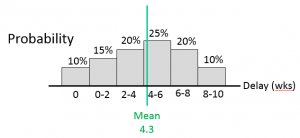
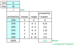
Figure 1: Delay Probability Analysis and Mean Calculation
Using this template we simply enter, into the blue cells, our best-case and worst-case scenarios, and the probabilities of these and a few increments between them. The probabilities add up to 100%, which indicates we have modeled all of the possibilities within this table. The mean is calculated by multiplying the probabilities by the impacts.
Once we have calculated the mean value, 4.3 weeks of delay in this example, then we use this value as expected delay (∆D). We could do the same for development expenses.
Notice, I haven’t included any probability that the activity will add more than 10 weeks to the schedule. As we learn from Theory of Constraints, for many reasons, completing activities later than expected is more likely than completing them early. The distribution is not normal, but instead has a long tail. Certainly sometimes it seems like things take forever. However, when we use economic analysis and have a lean development system, our durations are more in control so the tail is shorter. We complete tasks more quickly and see clearly when it is time to cut-bait and move on.
Accounting for Uncertainty in Sales Volume Gains
A similar probability analysis can be performed for the sales impact (gain), of the feature. Say, for this example, there is a small (10%) chance we will end up getting no value out of the feature because we have issues implementing it and need to cut bait. The probability of success, or its inverse, the probability of failure rather, is indicated in orange in the image below.
However, in this example, even if we are successful in our implementation, there is still another 10% probability we will get no sales increase from this decision. Perhaps there is a 5% chance that the customer will not value it, and a 5% chance that our competition will quickly counteract or duplicate our new capability.
Putting all of these scenarios into a single probability of no value is easier than trying to determine which apply to probability of success and which apply to the gain value.
For this example, in the best case, we expect an 8% volume improvement, and we think we are most likely to see a 5% volume increase, as indicated by our original estimate. We can easily accommodate all of these scenarios at the same time using probability analysis.
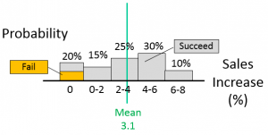

Figure 2: Sales Volume Change Probability Analysis and Mean Calculation
The probability of success (or failure, rather), is included in the calculation of the mean. In this case, it is included in the value for expected volume change (∆V), which we estimate now at 3.1%, rather than the 5% we think to be most likely. This makes it easy to enter into our comprehensive EV calculation.
Economic Value and Return on Investment Results
In our example, the EV would then be calculated as:
EV = 3.1% * $150K per % + SPS * 0 - 4.3 weeks * $100K per week + UCS * 0 - $16K
= $19K
And our Return on Investment is:
EROI = EV/∆E
= $19K/$16K
~= 1-to-1
This is much lower than the ROI we would get with our most likely estimate, which is a 5% sales gain.
EV = 5% * $150K per % - 4.3 weeks * $100K per week - $16K
= $304K
EROI = EV/∆E
= $304K / $16K
~= 19-to-1
This illustrates another of the many benefits of analyses. When people are asked to estimate how much a variable will be impacted (e.g., how much a feature will increase sales volume or delay launch), they often provide their most likely estimate. However, when we account for other possible impacts, we sometimes find that our decision changes.
Often the worst-case scenarios are bad enough to override both the best-case and the most-likely scenarios. Using a probability analysis is how we avoid those losing situations.
Comparing EMV to EV
EMV and EV are really two different ways to calculate the same thing. Evaluating the previous example in EMV terms give us the same answer. The mean gain we would receive if we are successful is the mean value of the grey areas only.
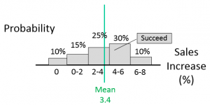
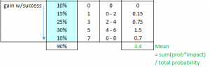
Figure 3: Mean Gain Value for EMV calculation
Then, the expected gain is the probability of success (90%) times the mean gain if we are successful (3.4%), resulting in an expected gain of 3.1% (3.4 * 90%). This is the same value from our probability analysis where probability of failure is included.
Importance of Certainty in Estimates
The previous example also demonstrates the importance of having good estimates for our Economic Variables. Where a 5% volume increase would result in $300K profit and a 19-to-1 ROI, a 3% increase is essentially a wash.
It is true that the age old adage of garbage in, garbage out, applies to economic analyses -- in some ways anyway. As discussed in part 6, imperfect volume forecasts and the resulting sensitivities and cost of delay do not necessarily invalidate these analyses. In this example, if our COD and SVS are actually half of the current estimates because our volume forecast was overestimated, the result is pretty much the same:
EV = 3.1% * $75K per % – 4.3 weeks * $50K per week – $16K
~= $1.5K
The difference between an economic value of $19K and $1.5K is very small relative to the profit gains we will see in some of our decisions, which are often in the hundreds of thousands or millions. Initiatives with an economic value of a few thousand dollars are too small to bother with, and we would decide in both cases not to pursue the new feature.
Summary
Accuracy in our Economic Variable mean estimates is often important, but not always. Sometimes, even our worst-case estimates give us a clear answer that differs from our initial intuition. Thus, sometimes we make better decisions and increase our profitability regardless of how accurate our mean estimates are. Nonetheless, in cases where we are on the bubble, the more accurate our impact estimates are, the more profitable our decisions will be.
However, as discussed in the post about how Economic Decision Making relates to Moneyball, making many decisions every week in product development means we realize the benefits of the law of large numbers and variability pooling. Over-estimates in one decision will generally be counteracted with underestimates in another. We don’t need to be perfect every time to be better, on average, and more profitable overall.
The better we can be at estimating the impacts of each decision, the more profitable our decisions will be. While product development will always be uncertain in many ways, as we can never predict the future with 100% accuracy, we are getting much better. In the next post we will discuss ways to achieve greater accuracy in the estimated impacts of our decisions, our Economic Variables. Stay tuned....
-----
Want to learn more about how to calculate cost of delay? Download the eBook.

Related Posts
Introduction to Cost of Delay
What is Cost of Delay?
Cost of Delay: How to Calculate It
Cost of Delay and Project Modeling
Cost of Delay Project Model Examples
Cost of Delay Project Modeling Risk
Cost of Delay and Strategic Advantage
Cost of Delay: Project decisions based on profit
8 Ways to Decrease Risk in Project Decisions
14 Tips for Calculating Cost of Delay
WSJF and How to Calculate It
Don Reinertsen on cost of delay
Wikipedia on cost of delay
Guide to Cost of Delay
Editor's note: This post was originally published in 2015 and has been updated for accuracy and comprehensiveness.
